A quick tour of Variational Autoencoder (VAE)

In recent times the generative model has gained huge attention due to its state-of-art performance and hence achieved massive importance in the marketplace and is also used widely. Variational Autoencoders are deep learning techniques used to learn the latent representations they are one of the finest approaches to unsupervised learning. VAE shows exceptional results in generating various kinds of data.

Autoencoder (AE) at a glance

Autoencoder comprises an encoder, decoder, and a bottleneck. The encoder simply transforms the input into a digital representation to the lowest dimension into the bottleneck to absorb its salient features and the decoder reconstructs back the output from the representations nearly similar to the input.

The Autoencoder aims to minimize the reconstruction loss. The reconstruction loss is the difference between the original data and the reconstructed data.

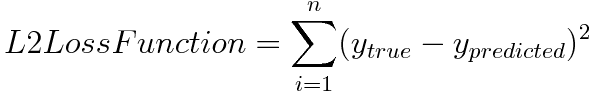
L2 Loss function is used to calculate the loss in AE. i.e the sum of all the squared differences between the true value and the predicted value.

The applications of an Autoencoder include Denoising, Dimensionality Reduction, etc.

Variational Autoencoders at a glance

VAE is also a kind of Autoencoder which not only reconstructs the output but also generates new content. Stating explicitly, VAE is a generative model and Autoencoders are not. The Autoencoder learns to transform an input into some vector representation by minimizing the reconstruction loss calculated from the input and the reconstructed image, VAE, on the other hand, generates output by minimizing the reconstruction as well as theKL Divergence loss which is the difference between the actual and observed probability distribution, It is the symmetrical score as well as the distance measure between two probabilistic distributions, in terms of VAE it tells whether the distribution learned is not far from a normal distribution.

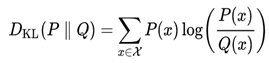
The above is the k-l divergence between distributionsP and Q over the space χ

Variational autoencoder can be defined as an autoencoder whose training is regularized to avoid overfitting problems and it makes sure that the latent space assimilates fruitful results that generate some distinctive and unique results.

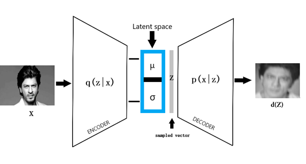
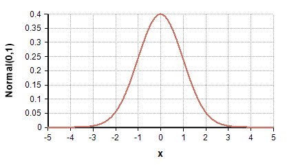
The variational autoencoder consists of an encoder, decoder, and a loss function. The encoder and decoder are simple neural networks. When input data X is passed through the encoder, the encoder outputs the latent state distributions (Mean μ, Variance σ) from which a vector is sampled Z. We always make an assumption that the latent distribution is always a Gaussian distribution. The input x is compressed by the encoder into a smaller dimension. Which is typically referred to as bottleneck or the latent space. From which some data is randomly sampled and the sample is decoded by backpropagating the reconstruction loss and we get a new generated variety.

Reparameterization Trick

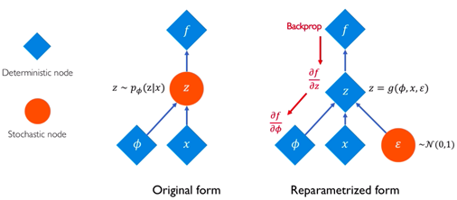
After the distribution is thrown out of the encoder, the sample is chosen by a random node which cannot make backpropagation possible. We need to backpropagate the encoder-decoder model to make it learn. To overcome the backpropagation, we use the epsilon (ε) with the mean and variance to maintain the stochasticity. So, at a time we can also choose a random sample and also learn with the latent distribution states. During the iterations, the epsilon remains the random sample and the parameters of the encoder output are updated.

After the distribution is thrown out of the encoder, the sample is chosen by a random node which cannot make backpropagation possible. We need to backpropagate the encoder-decoder model to make it learn. To overcome the backpropagation, we use the epsilon (ε) with the mean and variance to maintain the stochasticity. So, at a time we can also choose a random sample and also learn with the latent distribution states. During the iterations, the epsilon remains the random sample and the parameters of the encoder output are updated.

Implementation

Let try to implement the VAE into our code with MNIST data using PyTorch.

Install PyTorch with Torchvision

#command line>> pip3 install pip install torch==1.7.1+cpu torchvision==0.8.2+cpu torchaudio===0.7.2 -f https://download.pytorch.org/whl/torch_stable.html>> pip3 install numpy

Import Libraries

import torchvision.transforms as transformsimport torchvision

from torchvision.utils import save_imagefrom torch.utils.data import DataLoaderimport torchimport numpy as npimport torch.nn as nnimport torch.optim as optim

Prepare Data

We are using the MNIST dataset, so we’ll transform it by resizing it to 32x32 and converting it to tensor. Make data ready with the best ever PyTorch data loader with batches of 64

transform = transforms.Compose([transforms.Resize((32,32)),transforms.ToTensor(),])trainset = torchvision.datasets.MNIST(root='./', train=True, download=True, transform=transform)trainloader = DataLoader(trainset, batch_size=64, shuffle=True)testset = torchvision.datasets.MNIST(root='./', train=False, download=True, transform=transform)

MNIST Images have a single channel with 28x28 pixels.

define device to be used as per our requirement

dev = torch.device("cuda:0" if torch.cuda.is_available() else "cpu")

Define Loss function

def final_loss(bce_loss, mu, logvar):    BCE = bce_loss 
    KLD = -0.5 * torch.sum(1 + logvar - mu.pow(2) - logvar.exp())
    return BCE + KLD

The Loss is the sum of the Kullback-Leibler divergence and Binary Cross-Entropy

Define parameters

z_dim =20lr = 0.001criterion = nn.BCELoss(reduction='sum')epochs = 1batch_size = 64

Create Variational Autoencoder model

The Encoder consists of convolution, batch normalization layers with leaky relu. The output of the Encoder is the mean vector and the standard deviation vector.

import torch
import torch.nn as nn

class VAE(nn.Module):
    def __init__(self, z_dim):
        super(VAE, self).__init__()
        
        # Encoder
        self.conv1 = nn.Conv2d(1,   8, 4, stride=2, padding=1)
        self.bn1   = nn.BatchNorm2d(8)
        self.af1   = nn.LeakyReLU()
        
        self.conv2 = nn.Conv2d(8,  16, 4, stride=2, padding=1)
        self.bn2   = nn.BatchNorm2d(16)
        self.af2   = nn.LeakyReLU()
        
        self.conv3 = nn.Conv2d(16, 32, 4, stride=2, padding=1)
        self.bn3   = nn.BatchNorm2d(32)
        self.af3   = nn.LeakyReLU()
        
        self.conv4 = nn.Conv2d(32, 64, 4, stride=2, padding=0)
        self.bn4   = nn.BatchNorm2d(64)
        self.af4   = nn.LeakyReLU()
        
        # Bottleneck (FC for μ and log σ²)
        # Note: after conv4 on a 1×1 input, feature map is [batch, 64, 1, 1] → flatten to 64
        self.fc1      = nn.Linear(64, 128)
        self.fca1     = nn.LeakyReLU()
        self.fcd1     = nn.Dropout(0.2)
        
        self.fc_mu    = nn.Linear(128, z_dim)
        self.fc_logvar= nn.Linear(128, z_dim)
        self.fca2     = nn.LeakyReLU()
        self.fcd2     = nn.Dropout(0.2)
        
        # Decoder
        self.fc2   = nn.Linear(z_dim, 64)
        self.da1   = nn.LeakyReLU()
        self.dd1   = nn.Dropout(0.2)
        
        # Upsample + deconv blocks
        self.deu1  = nn.UpsamplingNearest2d(scale_factor=2)
        self.dec1  = nn.ConvTranspose2d(64, 64, 4, stride=2, padding=0)
        self.deb1  = nn.BatchNorm2d(64)
        self.dea1  = nn.LeakyReLU()
        
        self.deu2  = nn.UpsamplingNearest2d(scale_factor=2)
        self.dec2  = nn.ConvTranspose2d(64, 32, 4, stride=2, padding=1)
        self.deb2  = nn.BatchNorm2d(32)
        self.dea2  = nn.LeakyReLU()
        
        self.deu3  = nn.UpsamplingNearest2d(scale_factor=2)
        self.dec3  = nn.ConvTranspose2d(32, 16, 4, stride=2, padding=1)
        self.deb3  = nn.BatchNorm2d(16)
        self.dea3  = nn.LeakyReLU()
        
        self.deu4  = nn.UpsamplingNearest2d(scale_factor=2)
        self.dec4  = nn.ConvTranspose2d(16,  1, 4, stride=2, padding=1)
        self.dea4  = nn.Sigmoid()

The random vector is sampled out from the mean vector and the standard deviation. which is further reconstructed by applying upsampling and ConvTransposed layers, I used both the upsampling and ConvTransposed it gave me better results.

def sampling(self, mu, log_var):
    std = torch.exp(log_var / 2)
    epsilon = torch.randn_like(std)
    return mu + epsilon * std


def forward(self, x):
    # ——— Encoder ———
    x = self.conv1(x)
    x = self.BN1(x)
    x = self.af1(x)

    x = self.conv2(x)
    x = self.BN2(x)
    x = self.af2(x)

    x = self.conv3(x)
    x = self.BN3(x)
    x = self.af3(x)

    x = self.conv4(x)
    x = self.BN4(x)
    x = self.af4(x)

    # Flatten
    x = x.view(x.size(0), -1)

    # Fully-connected to latent parameters
    x_fc = self.fc1(x)
    mu = self.fc_mu(x_fc)
    mu = self.fca1(mu)
    mu = self.fcd1(mu)

    log_var = self.fc_log_var(x_fc)
    log_var = self.fca2(log_var)
    log_var = self.fcd2(log_var)

    # Reparameterize
    z = self.sampling(mu, log_var)
    z = self.fc2(z)
    z = self.da1(z)
    z = self.dd1(z)

    # Reshape for decoder
    z = z.view(-1, 64, 1, 1)

    # ——— Decoder ———
    d = self.dec1(z)
    d = self.deb1(d)
    d = self.dea1(d)

    d = self.dec2(d)
    d = self.deb2(d)
    d = self.dea2(d)

    d = self.dec3(d)
    d = self.deb3(d)
    d = self.dea3(d)

    d = self.dec4(d)
    reconstruction = self.dea4(d)

    return reconstruction, mu, log_var


# Configure device
device = dev
model = VAE().to(device)

# Define optimizer
optimizer = optim.Adam(model.parameters(), lr=lr)

# Tracking
grid_images = []
train_losses = []
valid_losses = []

def validate(model, dataloader, dataset, device, criterion):
    model.eval()
    running_loss = 0.0
    counter = 0
    recon_images = None

    with torch.no_grad():
        for i, data in tqdm(enumerate(dataloader), total=len(dataset) // batch_size):
            counter += 1
            imgs = data[0].to(device)

            reconstruction, mu, logvar = model(imgs)
            bce_loss = criterion(reconstruction, imgs)
            loss = final_loss(bce_loss, mu, logvar)
            running_loss += loss.item()

            # save the last batch for visualization
            if i == (len(dataset) // batch_size) - 1:
                recon_images = reconstruction

    val_loss = running_loss / counter
    return val_loss, recon_images


def train(model, dataloader, dataset, device, optimizer, criterion):
    model.train()
    running_loss = 0.0
    counter = 0

    for i, data in tqdm(enumerate(dataloader), total=len(dataset) // batch_size):
        counter += 1
        imgs = data[0].to(device)

        optimizer.zero_grad()
        reconstruction, mu, logvar = model(imgs)

        bce_loss = criterion(reconstruction, imgs)
        loss = final_loss(bce_loss, mu, logvar)
        loss.backward()
        optimizer.step()

        running_loss += loss.item()

    train_loss = running_loss / counter
    return train_loss


# Main training loop
for epoch in range(epochs):
    train_epoch_loss = train(
        model, trainloader, trainset, device, optimizer, criterion
    )
    valid_epoch_loss, recon_images = validate(
        model, testloader, testset, device, criterion
    )

    train_losses.append(train_epoch_loss)
    valid_losses.append(valid_epoch_loss)

    # save and visualize reconstructions
    save_image(recon_images.cpu(), f"./output_{epoch}.jpg")
    image_grid = make_grid(recon_images.detach().cpu())
    grid_images.append(image_grid)

    print(f"Epoch {epoch+1}/{epochs} — Train Loss: {train_epoch_loss:.4f}, Val Loss: {valid_epoch_loss:.4f}")

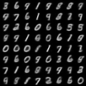
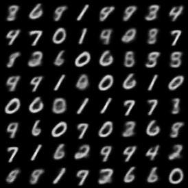
Here our model is trained and our reconstructed Images get saved into the defined path. The image below is the reconstructed Image I got after 5 epochs.

Model Prediction

Thing to Try

Try to reconstruct an image using your own custom-made image data. Hope you may get some surprising results, just try to Hypertune the model with different combinations. Try to increase the number of epochs. Try to play with the Z dim, learning rate, the convolution layers, strides, and much more.

Conclusion

VAE can perform much more if lots of data and proper computing power are used.

References

arxiv.org, medium.com